


Premium Support Included
In addition to providing the easiest way to get to your VPS and dedicated server through our unique features, Infosaic also provides a very robust control panel that allows you to take care of most of your advanced configuration needs.